CSDID Version 1.6

Prolog

CSDID v1.6 is here!. Not much change with respect to v1.5, but some improvements have been made. Namely, some improvements of efficiency, I added the WB Confidence intervals, and the option seed so one can replicate results.

The other addition. A simple csdid_plot. It is still quite limited, but it will allow you to make plots for event studies (like event_plot does), as well as plotting group ATT's and Calendar ATT's. Also, if you combine the results with Ben Jann's addplot, you can customize the results quite easily!.

For my own notes, and perhaps your understanding, A very quick revision of what CSDID and its "friend" DRDID do. You can skip the next section, if you are just interested in how CSDID works.

DID design

As it has been explained extensively, the TWFE model is not an appropriate method to identify ATT if the treatment effects are heterogeneous and the timing of the treatment varies across units.

There are now many papers that explain in detail why this is the case. I do my own version explain this (see on the left), but the bottom line is as follows. When you estimate a model like the following:

y_{it} = a_i + b_t + \theta (trt_i * post_t) + e_{it}

The parameter $\theta$ tries to estimate an average difference comparing the same unit across time, (one of the Differences), as well as comparing different units, with and without treatment, in the same point in time.

To my understanding, the first difference (changes across time), its still a good first approach. In fact, the way Sant'Anna and Zhao (2020) doubly robust estimator (implemented in DRDID) operates when using panel data is to estimate the within unit difference first, before using reweighthing methods to estimate the ATT.

Now, the second difference is problematic. First, one should understand what groups are being compared:

Treated units vs Never treated units: These are good comparisons
Treated units vs not yet treated units: These are also good, unless you think there are anticipation problems.
Later treated units vs earlier treated units: These are the bad ones. Because you are using as controls observations that were already treated.

Why is the third kind of comparison a bad average?

Perhaps saying "bad" is harsh. A better word would be a "potentially innapropriate comparison". So when is it a bad one, and when is it not?

Not so bad

If you believe that the treatment effect is homogenous, and has a one time shock on the outcome (in other words a one time shift upwards on the potential outcomes), then the standard TWFE is appropriate. Even comparison 3 is non problematic, and the earlier treated units are good "controls".

Definately bad

If you believe the treatment effects is heterogenous, and further more it changes across time, then the third comparison is innappropriate. Why? because we do not know how the earlier treated unit got affected.

Why is this important?.

Assume for a second that you have 2 observations, and that the parallel trend assumption hold for all before treatment. If one unit gets treated earlier, and the effect changes across time, then after treatment, its new "outcome trend" will NOT be parallel with the second unit. So, by the time the second unit is treated, you cannot compare it with the first (post treatment), because the parallel assumption does no longer holds!.

What about negative weights?!

Another way that has been discussed regarding the problems with TWFE has been the generation of Negative weights. For a while, this didn't strike me as an intuitive concept, but this problem is closely related to the bad groups comparisons. Let me try to explain, relaxing a bit of the rigourous math.

When you estimate ATT's, at the end of the day you are simply comparing Treated units vs untreated ones:

ATT =\sum \left( w1 * Y(treated,t) - w0 * Y (untreated,t) \right)

In this simple case, all treated receive a positive weigth, and all untreated units have an effective "negative" weight, because they need to be substracted.

Now, if you compare earlier treated units and later treated units you have the following:

ATT =\sum \left( w1 * Y(treated,t) - w0 * Y (treated earlier,t) \right)

Because the "earlier" treated unit is used as control, it is entering the equation substracting from the later treated one. However, at time t, it has already been treated, so it is receiving a "negative" weight!, when it should be possitive. And this is the source of the problem. TWFE would put "negative" weights on some treated units, because it uses them as "controls".

So what is the solution?

The solution, as you may suspect, is to simply avoid bad comparisons. And, yes, this is what Callaway and Sant'Anna (2021) does. It estimates all possible "good" comparisons for the estimation of ATT's, and then simply aggregates them to provide a summary of the results. But that is just half of the work.

The other half of the job is to actually estimate the treatment effects the best way possible, accounting for as much information as reasonable. This, as Pedro would say, is the building block that was proposed on his earlier work in Sant'Anna and Zhao (2020).

So why was the older `CSDID` slow?

As I mentioned before, CSDID works together with DRDID to obtain the best estimate for treatment effects. In essence DRDID estimates what is call the $ATT(g,t)$ , which is simply the Average treatment effect on the treated, for group $g$ (when the group gets treated) measure at time $t$ . Setting all the additional refinements of the doubly robust estimators, when $t \geq g$ , this is simply estimated as:

ATT(g,t) = \bigg[ EY(g)_t-EY(NT)_t \bigg] - \bigg[ EY(g)_{g-1}-EY(NT)_{g-1} \bigg]

Here, NT stands for "never treated", which can almost always be used a good control group. $EY(c)_t$ is the expected value of the oucome at time $t$ , for group $c$ . The first parenthesis calculates the differences in outcomes at time $t$ , while the second parenthesis estimates the outcome difference at time $g-1$ , which is the period before the treatment took place.

When $t < g$ , the $ATT(g,t)$ are simply defined as:

ATT(g,t) = \bigg[ EY(g)_t-EY(NT)_t \bigg] - \bigg[ EY(g)_{t-1}-EY(NT)_{t-1} \bigg]

Which can be used to check if the parallel trends assumptions hold by looking if the period-to-period outcome changes.

Now, you can see that this easily creates a large number of potential $ATT's$ to look at. Some could be interesting, but some would be too small to say anything about them. Here is where the step aggregation comes.

For any of the aggregations proposed in Callaway and Sant'Anna (2021), the general formula is:

AGGTT = \frac{\sum ( w_{g,t} * ATT(g,t))}{\sum ( w_{g,t})}

where $w_{g,t}$ is a weight of how much information was used to estimate $ATT(g,t)$ . Larger and more precise estimators should receive more weights, whereas those based on just a handful of observations, should be downweighted.

To obtain standard errors for this parameter, we need to rely on the delta method, differentiating the above expression with respect to each $ATT(g,t)$ and each $w_{g,t}$ . Needless to say, it can become a very long expression to keep track of.

In the previous iteraton of CSDID, this was done using nlcom. nlcom uses the delta method to estimate SE for nonlinear combination of parameters. It is usally pretty fast, but when you are trying to evaluate expressions with a large number of parameters, it can turn slow pretty quickly. Furthermore, there is a limit of how many equations you can tell nlcom to keep track. A few people contacted me already reporting this problem.

Is there a solution?

Yes, whenever there is a problem, there is a solution. Afterall, R's DID can do it, why can't I (and Stata). So that is what took some time to figure out. I simply needed to correctly track what elements enter a particular aggregation, and then multiply matrices, and summarize the Variance Covariance Matrix using the good old Sandwich Formula.

Var(AGGTT) = H' * \Omega * H

H = \left[ \begin{matrix} \frac{\partial AGGTT}{\partial ATT(g,t)} \\ \\ \frac{\partial AGGTT}{\partial w_{g,t}}\end{matrix} \right]

where $\Omega$ is the variance convariance for all the $ATT(g,t)$ and the $w_{g,t}$ .

Setup

Alright, the previous section was more of a brief introduction on the magic behind CSDID and DRDID. But now what you are really here for. The new CSDID.

First, in order to use CSDID you will need five sets of files:

drdid.ado. This is the workhorse of the estimation. Implements the 2x2 DID estimation for any possible pair of treated and untreated groups, as gets the Recentered Influence functions. This is what is used to make Statistical inferences. This implements Sant'Anna and Zhao (2020).
csdid.ado. This is the main program that implements Callaway and Sant'Anna (2021). It will call on drdid.ado, and put all the attgt's into a nice table. Itdoes the work that att_gt does. It does come with couple of new surprises.
csdid_estat.ado. This file will be used as a post-estimation program. It does the work that aggte and summarize does. And it now does it quickly, because it only uses the info left by csdid.
csdid_stats.ado. This is a new program that joins the CSDID family. (It may still recive a name change). This program will do mostly the same that csdid_estat.ado does, with a small difference. It will not work on your current dataset, it will work on a new dataset that you can create and store all the Influence functions created in CSDID. This is my attempt to simulate R's capacity to "save" entire datsets within objects for later use.
csdid_table.ado. This program works whenever wboot is called. It simply posts the Wildbootstrap confidence intervals.
csdid_plot.ado. This is the newst companion to the csdid package. A dedicated plotting command. It is simple to use, but it does impose a few restrictions on how much you want to modify on the plots. However, if you use addplot by Ben Jann, you can get very nice plots, quite easily.

In contrast with DID, my command uses drimp as the default estimator method. However, all other estimators within drdid will be allowed (except all and stdipwra). They key is to declare the method using option method(). Interestingly enough, DID uses dripw as the default. So I will use that for the following replication.

Simple Help file

Yes, I promise, at some point a proper helpfile will be created.

csdid

The general syntaxis of the command will be as follows:

csdid depvar indepvar [if] [in] [iw], ivar(varname) time(year) gvar(group_var) ///
        method(drdid estimator) [notyet] [saverif(file) replace cluster(varname) ///
        wboot agg(aggregation method) reps(#) rseed(#) wbtype(wbtype)]

Here an explanation of all the pieces:

depvar : is your dependent variable or outcome of interest
indepvar: are your independent variables, you may or may not have variables here. These variables will be included in the outcome regression specification and/or the propensity score estimation. Ideally, this are time constant variables. But time varying variables are allowed. In those cases, ATT's are estimated using pre-treatment values.
ivar: is a variable that identifies the panel ID. If you drop this, the command will use repeated crossection estimators instead. If included, it will estimate the panel estimators. If you use `ivar', you will need to have a proper panel data setup, with only one observation per ID per period.
time: identifies the time variable (for example year). It does not matter if the periods are contiguous or not. This variable should overlap all possible periods within `gvar'.
gvar: is a variable that identifies the first time an observation is treated. It should be within the "time" bracket. Observations with gvar==0 are considered never treated units.
method(estimator) is used to indicate which estimator you want to use. Below the list of all that is available:
- drimp Estimates the DR improved estimator. If you add rc1 it provides you with the alternative estimator (that is not locally efficient). Default
- dripw Estimates the DR IPW estimator. You can also use rc1 to provide the alternative (not locally efficient) estimator.
- reg Estimates the Outcome regression estimator.
- stdipw Estimates the Standard IPW estimator.
- ipw Estimates the estimator similar to Abadies (2005)
notyet request using not yet treated observations as controls, rather than never-treated observations only. This would imply a larger control group for the estimation of the treatment effects.

New options:

saverif(new file): This option allows you to save all the Recentered Influence functions created by CSDID into a new datafile. If you are familar with the ster files in Stata, this file will work in a similar way, where important information left by CSDID is stored for later use. It requires you to provide a new file name. It can be combined with replace, if the data-file already exists.
cluster(varname): You can use this to declare a variable to obtained clustered standard errors. If you declare ivar make sure that cluster remains constant within panel ID (cluster is nested)
wboot: This option requests the estimation of Wild Bootstrap Standard errors. When using this option, Covariances across parameters are not estimated. In the newest update, the correct CI are displayed.
reps(#): This allows you to choose how many repetitions you want to use for the WBootstrap SE. The default its 999.
rseed(#): With this, you can set a seed that would allow you to get replicable results. Of course, you can obtaine the same using set seed # before the command is excecuted.
wbtype(): You can now choose from two types of WB multipliers. The default is mammen, but you can also use rademacher.
agg(aggregation method): this option allows you to request csdid to directly produce any of the aggregations of interest, rather than report the attgt's. This can be combined with wboot, and saverif(). In all cases, however, I recommend using the saverif() option to keep a copy of the RIFs, for later inspection, even if you want to produce any aggregations from the start.

csdid_estat

This program works on the background to obtain all aggregations. This command will always estimate SE for aggregations using the analytical VCOV matrices, even if you request Wbootstrap estimations in csdid. If you want the Wbootstrap estimates, you can use csdid_stats, or use the agg() after csdid.

estat [subcommand], [estore(name) esave(name) replace *]

And this are the options:

pretrend: This tests if all the pre-treatment effects are all equal to 0.
simple: Estimates the simple aggregation of all post treatment effects.
group: Estimates the group average treatment effects
calendar: Estimates the calendar time average treatment effects
event: Estimates the dynamic aggregation/event study effects. If you use event, it is also possible to combine it with :
- , window(#1 #2): With this option, you can request to produce only a subset of all the posible dynamic effects.
estore(name): It allows you to save output table as an estimation equation.
esave(name): It allows you to save output table as an ster file. It can be combined with replace.
all: This produces all statistics.

All comands after estat, with the exception of pretrend, leave an r(table) element, as well as r(b) and r(V) matrices.

csdid_stats

The purpose of this command is to do what csdid_estat does, but when you are using a file previosly saved using the option saverif(). It works pretty much the same as csdid_estat, except that you can request analytical standard errors, as well as WildBootstrap standard errors. Compared to csdid_estat, this may be slower because it reproduces all Standard errors directly from the RIFs.

csdid_stats [subcommand], [estore(name) esave(name) replace]

And this are the options:

simple: Estimates the simple aggregation of all post treatment effects.
group: Estimates the group average treatment effects
calendar: Estimates the calendar time average treatment effects
event: Estimates the dynamic aggregation/event study effects. If you use event, it is also possible to combine it with : estore(name): It allows you to save output table as an estimation equation.
esave(name): It allows you to save output table as an ster file. It can be combined with replace.
wboot: Request the Wbootstrap Standard errors. it can be combined with rseed(#), reps(#) and wbtype().

All comands, with the exception of pretrend, leave an r(table) element, as well as r(b) and r(V) matrices.

csdid_plot

This command is my alternative to event_plot and perhaps similar to DID's ggplot option. It can be used as a post estimation, after csdid, csdid_estat, and csdid_stats.

The general syntax is as follows:

csdid_plot , [style(styleoption) title(str) name(str) group(#) ///
							 ytitle(str) xtitle(str) ]

Most options are self exaplanatory:

-style. Allows you to change the style of the plot. The options are rspike (default), rarea, rcap and rbar. -title, ytitle, xtitle are all two way graph options to modify the title, xaxis title, and y axis title. -name, Use if you want to store a figure in memory. -group(#) Use only after reporting the attgt's. One needs to use the group number to plot the dynamic effects with respect that that group.

Replication

So lets see how this works. First, load the data, and estimate the model. To replicate the DID simple output, I will use method(dripw).

use https://friosavila.github.io/playingwithstata/drdid/mpdta.dta, clear

. csdid  lemp lpop , ivar(countyreal) time(year) gvar(first_treat) method(dripw)


............
Difference-in-difference with Multiple Time Periods
Outcome model  : least squares
Treatment model: inverse probability
------------------------------------------------------------------------------
             | Coefficient  Std. err.      z    P>|z|     [95% conf. interval]
-------------+----------------------------------------------------------------
g2004        |
 t_2003_2004 |  -.0145297   .0221292    -0.66   0.511     -.057902    .0288427
 t_2003_2005 |  -.0764219   .0286713    -2.67   0.008    -.1326166   -.0202271
 t_2003_2006 |  -.1404483   .0353782    -3.97   0.000    -.2097882   -.0711084
 t_2003_2007 |  -.1069039   .0328865    -3.25   0.001    -.1713602   -.0424476
-------------+----------------------------------------------------------------
g2006        |
 t_2003_2004 |  -.0004721   .0222234    -0.02   0.983    -.0440293     .043085
 t_2004_2005 |  -.0062025   .0184957    -0.34   0.737    -.0424534    .0300484
 t_2005_2006 |   .0009606   .0194002     0.05   0.961    -.0370631    .0389843
 t_2005_2007 |  -.0412939   .0197211    -2.09   0.036    -.0799466   -.0026411
-------------+----------------------------------------------------------------
g2007        |
 t_2003_2004 |   .0267278   .0140657     1.90   0.057    -.0008404     .054296
 t_2004_2005 |  -.0045766   .0157178    -0.29   0.771    -.0353828    .0262297
 t_2005_2006 |  -.0284475   .0181809    -1.56   0.118    -.0640814    .0071864
 t_2006_2007 |  -.0287814    .016239    -1.77   0.076    -.0606091    .0030464
------------------------------------------------------------------------------
Control: Never Treated

See Callaway and Sant'Anna (2021) for details

I find this output a bit easier to understand than the baseline output in R. Each equation represents the group treatment. And each coefficient represents the two years (pre and post) used to estimate the ATT.

All point estimates are the same as the R command. The standard errors are different, because R's DID uses Wbootstrap standard errors by default, whereas I use the asymptotic normal ones as default. You can replicate this in R using the bstrap = F option. In the previous version, you also saw the "weights" equations. They are still produced, but are no longer shown.

So what about the aggregation. The first thing would be the pretrend test for parallel assumption. The output is subject to change.

. estat pretrend
Pretrend Test. H0 All Pre-treatment are equal to 0
chi2(5) = 6.841824981670454
p-value       = .2326722805724242

We can also reproduce the simple, calendar and group aggregations:


. estat simple 
Average Treatment Effect on Treated
------------------------------------------------------------------------------
             | Coefficient  Std. err.      z    P>|z|     [95% conf. interval]
-------------+----------------------------------------------------------------
         ATT |  -.0417518   .0115028    -3.63   0.000    -.0642969   -.0192066
------------------------------------------------------------------------------

. estat calendar
ATT by Calendar Period
------------------------------------------------------------------------------
             | Coefficient  Std. err.      z    P>|z|     [95% conf. interval]
-------------+----------------------------------------------------------------
       T2004 |  -.0145297   .0221292    -0.66   0.511     -.057902    .0288427
       T2005 |  -.0764219   .0286713    -2.67   0.008    -.1326166   -.0202271
       T2006 |  -.0461757   .0212107    -2.18   0.029     -.087748   -.0046035
       T2007 |  -.0395822   .0129299    -3.06   0.002    -.0649242   -.0142401
------------------------------------------------------------------------------

. estat group
ATT by group
------------------------------------------------------------------------------
             | Coefficient  Std. err.      z    P>|z|     [95% conf. interval]
-------------+----------------------------------------------------------------
       G2004 |  -.0845759   .0245649    -3.44   0.001    -.1327222   -.0364297
       G2006 |  -.0201666   .0174696    -1.15   0.248    -.0544065    .0140732
       G2007 |  -.0287814    .016239    -1.77   0.076    -.0606091    .0030464
------------------------------------------------------------------------------

And the one that was the most difficult to program, but is the most interesting. The event study/dynamic effects:

. estat event
ATT by Periods Before and After treatment
Event Study:Dynamic effects
------------------------------------------------------------------------------
             | Coefficient  Std. err.      z    P>|z|     [95% conf. interval]
-------------+----------------------------------------------------------------
         T-3 |   .0267278   .0140657     1.90   0.057    -.0008404     .054296
         T-2 |  -.0036165   .0129283    -0.28   0.780    -.0289555    .0217226
         T-1 |   -.023244   .0144851    -1.60   0.109    -.0516343    .0051463
           T |  -.0210604   .0114942    -1.83   0.067    -.0435886    .0014679
         T+1 |  -.0530032   .0163465    -3.24   0.001    -.0850417   -.0209647
         T+2 |  -.1404483   .0353782    -3.97   0.000    -.2097882   -.0711084
         T+3 |  -.1069039   .0328865    -3.25   0.001    -.1713602   -.0424476
------------------------------------------------------------------------------

What If i wanted to get the event aggregation to begin with? I can do this, from the csdid command line. I can also store the RIF's in a new file. and request Wild Bootstrap Standard errors.

csdid  lemp lpop , ivar(countyreal) time(year) gvar(first_treat) method(dripw) ///
agg(event) saverif(rif_example) wboot replace rseed(1)
File rif_example.dta will be used to save all RIFs
............
(file rif_example.dta not found)
file rif_example.dta saved

Difference-in-difference with Multiple Time Periods
Outcome model  : least squares
Treatment model: inverse probability
----------------------------------------------------------------------
             | Coefficient  Std. err.      t      [95% conf. interval]
-------------+--------------------------------------------------------
         T-3 |   .0267278   .0145166     1.84    -.0004601    .0539157
         T-2 |  -.0036165   .0128202    -0.28     -.030182     .022949
         T-1 |   -.023244   .0152288    -1.53    -.0524744    .0059864
         T+0 |  -.0210604   .0118453    -1.78    -.0441373    .0020166
         T+1 |  -.0530032   .0161958    -3.27    -.0841509   -.0218555
         T+2 |  -.1404483    .036125    -3.89    -.2145895   -.0663072
         T+3 |  -.1069039   .0349244    -3.06    -.1711649   -.0426429
----------------------------------------------------------------------
Control: Never Treated

See Callaway and Sant'Anna (2021) for details

Now, I dont want to re-estimate this model again, but I'm interested in other aggregations, and able to save the RIF's from before. What I can do now is obtain the Wildbootstrap estimates.

.  use rif_example, clear

.  csdid_stats simple , wboot rseed(1)
----------------------------------------------------------------------
             | Coefficient  Std. err.      t      [95% conf. interval]
-------------+--------------------------------------------------------
         ATT |  -.0417518   .0111832    -3.73    -.0627803   -.0207233
----------------------------------------------------------------------

. csdid_stats calendar, wboot rseed(1)
----------------------------------------------------------------------
             | Coefficient  Std. err.      t      [95% conf. interval]
-------------+--------------------------------------------------------
       T2004 |  -.0145297   .0219889    -0.66    -.0582209    .0291616
       T2005 |  -.0764219    .026394    -2.90    -.1326498    -.020194
       T2006 |  -.0461757    .022042    -2.09    -.0886126   -.0037388
       T2007 |  -.0395822   .0119995    -3.30    -.0637637   -.0154006
----------------------------------------------------------------------

csdid_stats group, wboot rseed(1)
----------------------------------------------------------------------
             | Coefficient  Std. err.      t      [95% conf. interval]
-------------+--------------------------------------------------------
       G2004 |  -.0845759   .0239044    -3.54    -.1317318   -.0374201
       G2006 |  -.0201666   .0171841    -1.17    -.0541214    .0137881
       G2007 |  -.0287814   .0160165    -1.80    -.0590851    .0015224
----------------------------------------------------------------------

csdid_stats event, wboot rseed(1)
----------------------------------------------------------------------
             | Coefficient  Std. err.      t      [95% conf. interval]
-------------+--------------------------------------------------------
         T-3 |   .0267278   .0138167     1.93     .0007082    .0527474
         T-2 |  -.0036165   .0128959    -0.28    -.0298632    .0226302
         T-1 |   -.023244   .0145381    -1.60    -.0527278    .0062398
         T+0 |  -.0210604   .0114842    -1.83    -.0423346    .0002139
         T+1 |  -.0530032    .016063    -3.30    -.0844554    -.021551
         T+2 |  -.1404483   .0348762    -4.03    -.2097142   -.0711825
         T+3 |  -.1069039   .0315282    -3.39    -.1680153   -.0457924
----------------------------------------------------------------------

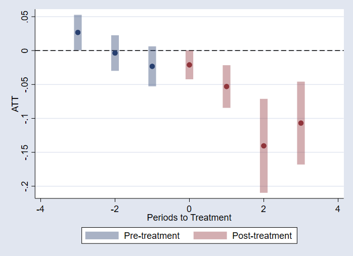
What about those graphs? Starting from the previous setup, I can re-estimate the event statistics, and then just call on csdid_plot.

qui:csdid_stats event, wboot rseed(1)
csdid_plot

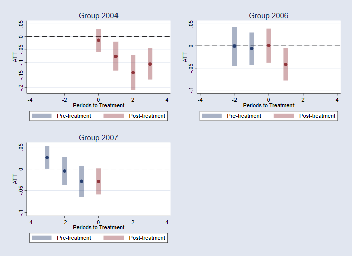
I could, however, do something similar but for the each cohort/group:

qui:csdid_stats attgt, wboot rseed(1)
csdid_plot, group(2004) name(m1,replace) title("Group 2004")
csdid_plot, group(2006) name(m2,replace) title("Group 2006")
csdid_plot, group(2007) name(m3,replace) title("Group 2007")
graph combine m1 m2 m3, xcommon scale(0.8)

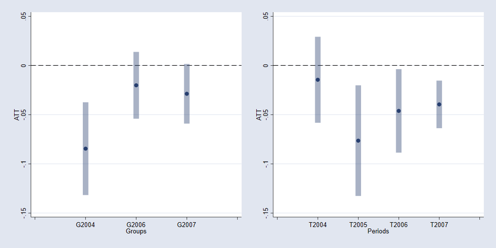
Or estimate the ATTS by cohort and year.

qui:csdid_stats group, wboot rseed(1)
csdid_plot, name(m1,replace) 
qui:csdid_stats calendar, wboot rseed(1)
csdid_plot, name(m2,replace) 
graph combine m1 m2, xcommon xsize(10) ysize(5)

And after this is done, you can use addplot (ssc install addplot) to do further figure edits.

What is next?

More stress testing. I have done a few more. Thanks to all the people reporting the different bugs and errors!
Some verification. Many data verifications have been added. But some checks may be missing. For instance, right now the command doesnt check if your weights are fixed for panel ID (which should be).
Help files. The hardest part...it seems. More flexible graphs! but that is for another time!